
Comparing proximity effects between conditions
Elijah Willie
2026-10-13
Source:vignettes/condition.Rmd
condition.RmdIntroduction
The PACE manual fits one section. This vignette asks whether a proximity effect differs between two groups of patients.
That needs a cohort, and adds one block to the model. Beside the spatial cell state block, the proximity effect common to both arms, PACE estimates a responder spatial state block: the part that differs between them.
The melanoma subset
The package ships a subset of a CosMx melanoma cohort of patients profiled after immune checkpoint blockade, contrasting progressive disease (PD) against non-progressive disease (non-PD, pooling stable, partial and complete responders).
library(PACE)
library(SpatialExperiment)
library(ggplot2)
library(dplyr)

spe <- readRDS(system.file("extdata", "mel_cosmx_subset.rds", package = "PACE"))
spe
#> class: SpatialExperiment
#> dim: 180 56274
#> metadata(0):
#> assays(1): counts
#> rownames(180): ANXA2 APOD ... WIF1 YBX3
#> rowData names(0):
#> colnames(56274): Cell52866 Cell52867 ... Cell21744 Cell21745
#> colData names(4): cellType Responder image sample_id
#> reducedDimNames(0):
#> mainExpName: NULL
#> altExpNames(0):
#> spatialCoords names(2) : x y
#> imgData names(0):
table(spe$cellType)
#>
#>      B_Cell Endothelial  Fibroblast  Macrophage      T_Cell      Tumour
#>        1129        1261        1488        3101        3406       45889
table(unique(data.frame(image = spe$image, arm = spe$Responder))$arm)
#>
#> nonPD    PD
#>    19     7
One section per patient, so the contrast is between patients.
Every cell and patient of the published cohort is here; only the
panel is reduced, to the 180 most detected of 927 genes. Derivation:
inst/scripts/make-mel-cosmx-subset.R.
Provenance. These data are a subset of the deposit accompanying Dong, Su, Kluger, Fan and Kluger, SIMVI disentangles intrinsic and spatial-induced cellular states in spatial omics data (doi:10.5281/zenodo.14708000), used here under CC-BY-4.0.
Fitting with a condition
Three arguments beyond the single-section call:
-
condition_colnames the contrast and switches on the responder block. -
kernel_per_image = TRUEkeeps neighbourhoods within a section, so no cell neighbours another patient’s. -
image_re = "intercept"absorbs patient-level shifts in overall expression.
fit <- paceFit(spe,
               celltype_col     = "cellType",
               condition_col    = "Responder",
               image_col        = "image",
               kernel_per_image = TRUE,
               image_re         = "intercept",
               dispersion       = "nb1",
               verbose          = FALSE)
#>  - Computing 180 x 298 likelihood matrix.
#>  - Likelihood calculations took 0.04 seconds.
#>  - Fitting model with 298 mixture components.
#>  - Model fitting took 0.25 seconds.
#>  - Computing posterior matrices.
#>  - Computation allocated took 0.00 seconds.
#>  - Computing 180 x 375 likelihood matrix.
#>  - Likelihood calculations took 0.05 seconds.
#>  - Fitting model with 375 mixture components.
#>  - Model fitting took 0.39 seconds.
#>  - Computing posterior matrices.
#>  - Computation allocated took 0.00 seconds.
#>  - Computing 180 x 579 likelihood matrix.
#>  - Likelihood calculations took 0.08 seconds.
#>  - Fitting model with 579 mixture components.
#>  - Model fitting took 0.68 seconds.
#>  - Computing posterior matrices.
#>  - Computation allocated took 0.00 seconds.
#>  - Computing 180 x 364 likelihood matrix.
#>  - Likelihood calculations took 0.05 seconds.
#>  - Fitting model with 364 mixture components.
#>  - Model fitting took 0.32 seconds.
#>  - Computing posterior matrices.
#>  - Computation allocated took 0.00 seconds.
#>  - Computing 180 x 243 likelihood matrix.
#>  - Likelihood calculations took 0.03 seconds.
#>  - Fitting model with 243 mixture components.
#>  - Model fitting took 0.23 seconds.
#>  - Computing posterior matrices.
#>  - Computation allocated took 0.00 seconds.
#>  - Computing 180 x 375 likelihood matrix.
#>  - Likelihood calculations took 0.05 seconds.
#>  - Fitting model with 375 mixture components.
#>  - Model fitting took 0.39 seconds.
#>  - Computing posterior matrices.
#>  - Computation allocated took 0.00 seconds.
#>  - Computing 180 x 364 likelihood matrix.
#>  - Likelihood calculations took 0.05 seconds.
#>  - Fitting model with 364 mixture components.
#>  - Model fitting took 0.20 seconds.
#>  - Computing posterior matrices.
#>  - Computation allocated took 0.00 seconds.
#>  - Computing 180 x 562 likelihood matrix.
#>  - Likelihood calculations took 0.08 seconds.
#>  - Fitting model with 562 mixture components.
#>  - Model fitting took 0.27 seconds.
#>  - Computing posterior matrices.
#>  - Computation allocated took 0.00 seconds.
#>  - Computing 180 x 265 likelihood matrix.
#>  - Likelihood calculations took 0.04 seconds.
#>  - Fitting model with 265 mixture components.
#>  - Model fitting took 0.31 seconds.
#>  - Computing posterior matrices.
#>  - Computation allocated took 0.00 seconds.
#>  - Computing 180 x 409 likelihood matrix.
#>  - Likelihood calculations took 0.06 seconds.
#>  - Fitting model with 409 mixture components.
#>  - Model fitting took 0.68 seconds.
#>  - Computing posterior matrices.
#>  - Computation allocated took 0.00 seconds.
fit
#> class: PACEFit
#> cell types (6): B_Cell, Endothelial, Fibroblast, Macrophage, T_Cell, Tumour
#> kernels: h_bio = 30 um, h_tech = 5 um | contamination: percell_hc; dispersion: nb1
#> condition: Responder (ResponderPD)
#> pipeline: model -> shrink -> decompose -> drivers
#>   neighbour slopes: 6480 rows (76 at lfsr < 0.05, 0.7 expected to have the wrong sign)
The interaction term is named from the non-reference level of
condition_col:
fit@params$resp_term
#> [1] "ResponderPD"
so ResponderPD:Tumour is the extra change in expression
per unit of tumour proximity in the PD arm, on top of the
Tumour effect shared by both arms.
The responder block in the decomposition
varianceDecomposition() now carries a
Responder spatial % column beside the
Spatial % one:
varianceDecomposition(fit) |>
  group_by(focal) |>
  summarise(`Spatial %`           = round(median(`Spatial %`), 4),
            `Responder spatial %` = round(median(`Responder spatial %`), 4),
            `Spillover %`         = round(median(`Spillover %`), 2),
            .groups = "drop")
#> # A tibble: 6 × 4
#>   focal       `Spatial %` `Responder spatial %` `Spillover %`
#>   <chr>             <dbl>                 <dbl>         <dbl>
#> 1 B_Cell            0.230                0.0005          12.1
#> 2 Endothelial       0.238                0.0242          13.9
#> 3 Fibroblast        0.343                0.0762          18.4
#> 4 Macrophage        0.478                0.025           19.6
#> 5 T_Cell            0.317                0.0019          13
#> 6 Tumour            0.307                0.034            3.2
The responder block is much the smaller: most of a cell’s response to its neighbours is common to both arms. Contamination exceeds both, and is largest in the sparse immune populations.
plotDecomposition() shows the same thing. On a fit with
a condition it adds a “Responder spatial state” block beside the shared
spatial one, so the two are directly comparable; on a fit without one
that block is simply absent. The right panel zooms in on the small
components, which are otherwise invisible next to cell-type
identity.
plotDecomposition(fit)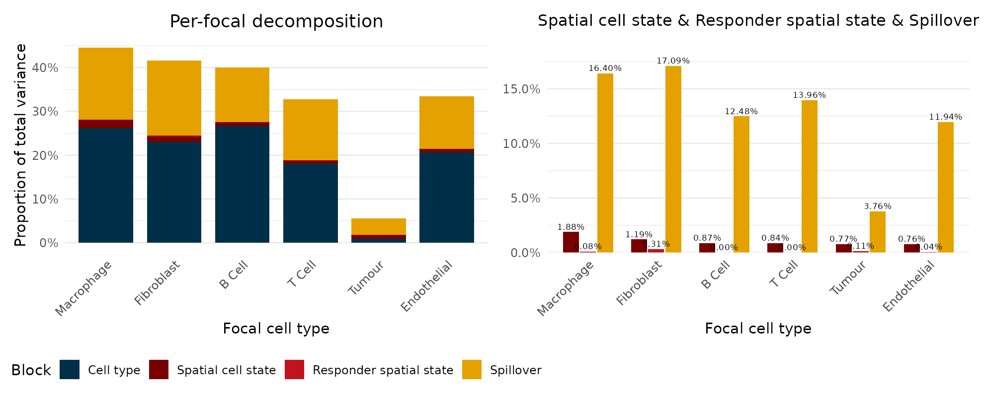
Which pairs carry the condition difference
pairVariance() and plotPairHeatmap() both
take block = "responder", which attributes the responder
block across neighbours instead of the shared spatial one:
pairVariance(fit, block = "responder") |>
  arrange(desc(val)) |>
  head(5)
#> # A tibble: 5 × 3
#>   focal      neighbour      val
#>   <chr>      <chr>        <dbl>
#> 1 Fibroblast Endothelial 0.271
#> 2 Tumour     Endothelial 0.0741
#> 3 Macrophage Fibroblast  0.0417
#> 4 Fibroblast Tumour      0.0380
#> 5 Macrophage Tumour      0.0365

plotPairHeatmap(fit, block = "responder")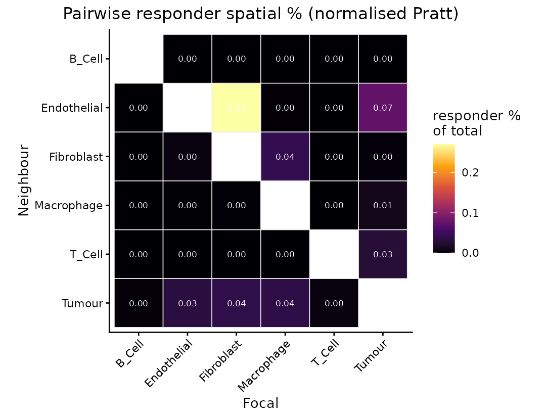
Fibroblast next to endothelium takes the largest share. Compare the shared spatial block, which orders differently:
plotPairHeatmap(fit, block = "spatial")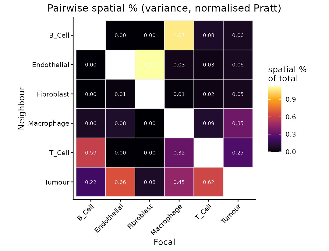
The genes that carry it
Pair shares say where to look, neighbourSlopes() which
genes. The ResponderPD: terms differ between arms:
ns <- neighbourSlopes(fit)
resp <- subset(ns, grepl("^ResponderPD:", term) & lfsr < 0.05)
nrow(resp)
#> [1] 76

resp[order(resp$lfsr), c("gene", "focal", "neighbour", "estimate_shrunk", "lfsr")] |>
  head(8)
#>        gene      focal   neighbour estimate_shrunk         lfsr
#> 2053   GLUL     Tumour Endothelial     -0.39965573 0.000000e+00
#> 6100   SPP1 Macrophage      Tumour     -0.06630620 0.000000e+00
#> 5351    MX1     Tumour      T_Cell      0.23157932 7.979372e-53
#> 5317 IFITM1     Tumour      T_Cell      0.18729859 4.405081e-33
#> 6373   GLUL     Tumour      Tumour      0.01628370 2.387829e-23
#> 5226    B2M     Tumour      T_Cell      0.10499260 6.530095e-23
#> 5383  STAT1     Tumour      T_Cell      0.14030844 2.374834e-22
#> 6401 IGFBP7     Tumour      Tumour      0.01674059 6.350817e-22
plotDrivers() gives a pair as a figure: the genes ranked
by driver score on the left, their per-gene decomposition on the right.
On a fit with a condition the score is built from the
resp_term interaction, so this ranks genes by how much the
proximity effect differs between arms, not by the
effect they share. Taking tumour cells next to T cells, CRYAB,
MZT2A and S100B lead, and nine of the thirteen genes
called are MHC class I or interferon: B2M, HLA-B,
HLA-C, HLA-E, STAT1, MX1,
IFITM1, IFITM3 and IFI27. Those nine all have
positive interactions, so their response to T cell proximity is steeper
in the progressive arm.
plotDrivers(fit, "Tumour", "T_Cell")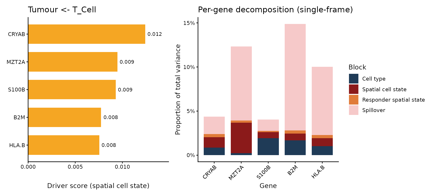
Two things follow from the score being the interaction. A difference
between arms subtracts anything common to both, and contamination from
the neighbour is largely common to both, so this ranking is less exposed
to it than a ranking of the shared effect would be. That matters here,
because B2M and HLA-B are expressed by T cells
themselves and the right panel shows spillover as their largest block;
it is the differencing, not the size of that block, that makes the
ranking readable. To rank the shared effect instead, re-run
paceShrink() with the responder term switched off, which
puts the shrinkage on the baseline slopes. No new model fit is
needed.
topDrivers() returns the same ranking as a table, with
the score and the parts it is built from:
topDrivers(fit)[["Tumour_T_Cell"]]$scores |>
  select(rank, gene, driver_score, b_clean, spec, focal_mean, lfsr) |>
  head(8)
#>   rank   gene driver_score     b_clean      spec focal_mean         lfsr
#> 1    1  CRYAB  0.012423231 -0.12157232 0.7873320  1.3559677 3.640576e-04
#> 2    2  MZT2A  0.009467803 -0.03143655 0.6203181 24.8972085 2.551249e-03
#> 3    3  S100B  0.009295063 -0.06493689 0.7937279  3.4988559 2.237826e-02
#> 4    4    B2M  0.007748198  0.10499260 0.3437164  5.9495304 6.530095e-23
#> 5    5  HLA.B  0.007548406  0.09946964 0.4063803  4.6196474 6.936858e-09
#> 6    6 IFITM1  0.006929811  0.18729859 0.4021399  1.2215128 4.405081e-33
#> 7    7  HLA.C  0.005827441  0.08250295 0.4333179  4.5595894 7.394678e-07
#> 8    8    MX1  0.005289734  0.23157932 0.3824699  0.6742792 7.979372e-53
The table is also filtered at lfsr < 0.05, so a
sparse figure means few genes cleared that threshold rather than few
genes being involved. On this reduced panel
Macrophage <- Tumour has only one, which is why the pair
shown here is a different one.
Among the strongest is SPP1 in macrophages next to tumour cells:
subset(ns, gene == "SPP1" & focal == "Macrophage" & neighbour == "Tumour")
#>      gene      focal neighbour               term    estimate   std.error
#> 6100 SPP1 Macrophage    Tumour ResponderPD:Tumour -0.06738867 0.006192822
#>      estimate_shrunk   sd_shrunk lfsr
#> 6100      -0.0663062 0.006056031    0
Tumour is the response shared by both arms;
ResponderPD:Tumour is how much it differs in progressive
disease. Negative, so macrophage SPP1 rises less steeply with
tumour proximity when disease progressed. This is the paper’s melanoma
result.
The counts behind it, split by arm:
plotProximity(fit, spe, "SPP1", "Macrophage", "Tumour",
              breaks = c(0, 10, 20, 30, 40, Inf), condition = TRUE)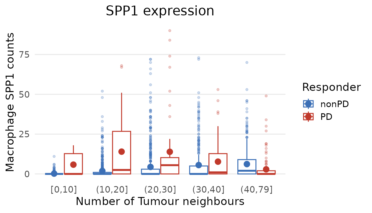
plotResponseCurve() puts the model over the data: solid
lines are binned means and standard errors, dashed lines the PACE slopes
read from the fit.
plotResponseCurve(fit, spe, "SPP1", "Macrophage", "Tumour")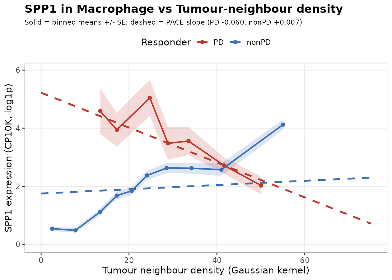
The dashed lines diverge; that divergence is the interaction. The x axis is the model’s own covariate, so the slopes are drawn on the scale they were estimated on.
plotResponseMap() gives the spatial view, using the two
sections shown in the paper:
plotResponseMap(fit, spe, "SPP1", "Macrophage", "Tumour",
                images = c(nonPD = "32157_18", PD = "32156_17"))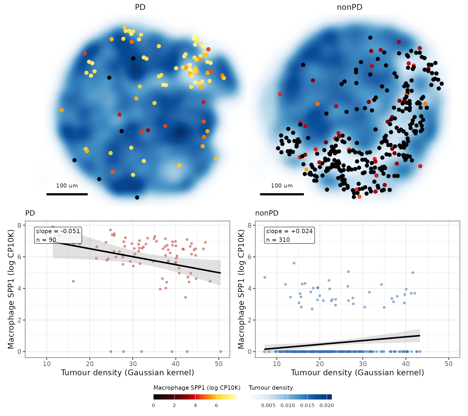
Session info
sessionInfo()
#> R version 4.6.1 (2026-06-24)
#> Platform: x86_64-pc-linux-gnu
#> Running under: Ubuntu 24.04.5 LTS
#>
#> Matrix products: default
#> BLAS:   /usr/lib/x86_64-linux-gnu/openblas-pthread/libblas.so.3
#> LAPACK: /usr/lib/x86_64-linux-gnu/openblas-pthread/libopenblasp-r0.3.26.so;  LAPACK version 3.12.0
#>
#> locale:
#>  [1] LC_CTYPE=C.UTF-8       LC_NUMERIC=C           LC_TIME=C.UTF-8
#>  [4] LC_COLLATE=C.UTF-8     LC_MONETARY=C.UTF-8    LC_MESSAGES=C.UTF-8
#>  [7] LC_PAPER=C.UTF-8       LC_NAME=C              LC_ADDRESS=C
#> [10] LC_TELEPHONE=C         LC_MEASUREMENT=C.UTF-8 LC_IDENTIFICATION=C
#>
#> time zone: UTC
#> tzcode source: system (glibc)
#>
#> attached base packages:
#> [1] stats4    stats     graphics  grDevices utils     datasets  methods
#> [8] base
#>
#> other attached packages:
#>  [1] dplyr_1.2.1                 ggplot2_4.0.3
#>  [3] SpatialExperiment_1.22.0    SingleCellExperiment_1.34.0
#>  [5] SummarizedExperiment_1.42.0 Biobase_2.72.0
#>  [7] GenomicRanges_1.64.0        Seqinfo_1.2.0
#>  [9] IRanges_2.46.0              S4Vectors_0.50.3
#> [11] BiocGenerics_0.58.1         generics_0.1.4
#> [13] MatrixGenerics_1.24.0       matrixStats_1.5.0
#> [15] PACE_0.99.11                BiocStyle_2.40.0
#>
#> loaded via a namespace (and not attached):
#>  [1] tidyselect_1.2.1    viridisLite_0.4.3   farver_2.1.2
#>  [4] S7_0.2.2            fastmap_1.2.0       digest_0.6.39
#>  [7] lifecycle_1.0.5     invgamma_1.2        magrittr_2.0.5
#> [10] dbscan_1.2.7        compiler_4.6.1      rlang_1.3.0
#> [13] sass_0.4.10         tools_4.6.1         utf8_1.2.6
#> [16] yaml_2.3.12         knitr_1.52          S4Arrays_1.12.1
#> [19] labeling_0.4.3      DelayedArray_0.38.2 plyr_1.8.9
#> [22] RColorBrewer_1.1-3  abind_1.4-8         withr_3.0.3
#> [25] purrr_1.2.2         desc_1.4.3          grid_4.6.1
#> [28] scales_1.4.0        MASS_7.3-65         cli_3.6.6
#> [31] mvtnorm_1.4-2       rmarkdown_2.32      ragg_1.5.2
#> [34] otel_0.2.0          rjson_0.2.23        cachem_1.1.0
#> [37] stringr_1.6.0       splines_4.6.1       assertthat_0.2.1
#> [40] BiocManager_1.30.27 XVector_0.52.0      vctrs_0.7.3
#> [43] Matrix_1.7-5        jsonlite_2.0.0      bookdown_0.48
#> [46] patchwork_1.3.2     mixsqp_0.3-54       irlba_2.4.1
#> [49] systemfonts_1.3.2   magick_2.9.1        jquerylib_0.1.4
#> [52] tidyr_1.3.2         glue_1.8.1          pkgdown_2.2.1
#> [55] stringi_1.8.9       gtable_0.3.6        rmeta_3.0
#> [58] tibble_3.3.1        pillar_1.11.1       htmltools_0.5.9
#> [61] truncnorm_1.0-9     R6_2.6.1            mashr_0.2.79
#> [64] textshaping_1.0.5   evaluate_1.0.5      lattice_0.22-9
#> [67] SQUAREM_2026.1      ashr_2.2-63         bslib_0.12.0
#> [70] Rcpp_1.1.2          nlme_3.1-169        SparseArray_1.12.3
#> [73] mgcv_1.9-4          xfun_0.61           fs_2.1.0
#> [76] pkgconfig_2.0.3