
Installation
if (!require("BiocManager")) install.packages("BiocManager")
BiocManager::install("remotes")
remotes::install_github("ecool50/PACE")
Introduction
PACE (Proximity-Associated Changes in Expression) is a framework for imaging-based spatial transcriptomics (such as Xenium and CosMx) that quantifies how a cell’s gene expression changes with proximity to specific neighbouring cell types. Rather than asking only which genes are spatially variable, PACE asks a directed question: when a macrophage sits next to tumour cells, which of its genes go up or down, and by how much?
PACE fits a hierarchical negative binomial mixed model with partial pooling across cell types, so that each focal-neighbour relationship borrows strength from the others and noisy pairs are regularised towards the consensus. A per-cell contamination term absorbs the short-range ambient signal that leaks between adjacent cells through segmentation error, so the estimated neighbour effect reflects biology rather than transcript misassignment.
Overview of the PACE workflow
A PACE analysis has three stages, all driven by the single call
paceFit():
- Neighbourhood construction. For every cell, a Gaussian biological kernel summarises the abundance of each neighbouring cell type, and a short-range exponential technical kernel captures the ambient contamination field.
- Model fitting. A streaming penalised quasi-likelihood fit estimates, for every gene and every focal cell type, a partially pooled slope on each neighbour type’s abundance, jointly with a per-cell contamination loading and gene-wise overdispersions. The neighbour slopes are then stabilised by multivariate adaptive shrinkage.
-
Interpretation. The fit is read out three ways:
shrunken neighbour slopes with a local false sign rate
(
neighbourSlopes()), a per-gene variance decomposition (varianceDecomposition()), and per-pair driver-score tables ranking the genes that mediate each relationship (topDrivers()).
The breast cancer dataset
The package ships a small worked example: a spatial crop of a human breast cancer Xenium section (10x Genomics; nucleus segmentation, cell types annotated with scClassify), centred on a tumour-macrophage interface. It contains 7,898 cells across eight cell types (B cell, dendritic cell, endothelial, macrophage, myoepithelial, stromal, T cell, and tumour) and a 278-gene panel, packaged as a SpatialExperiment. This region reproduces the macrophage reprogramming that PACE identifies on the full section.
library(PACE)
library(SpatialExperiment)
library(ggplot2)
library(dplyr)
library(tidyr)

spe <- readRDS(system.file("extdata", "bc_xenium_subset.rds", package = "PACE"))
spe
#> class: SpatialExperiment
#> dim: 278 7898
#> metadata(0):
#> assays(1): counts
#> rownames(278): SEC11C DAPK3 ... NOSTRIN CD1C
#> rowData names(0):
#> colnames(7898): 442 444 ... 99842 99848
#> colData names(2): cellType sample_id
#> reducedDimNames(0):
#> mainExpName: NULL
#> altExpNames(0):
#> spatialCoords names(2) : x y
#> imgData names(0):
table(spe$cellType)
#>
#>         B_Cell Dendritic_Cell    Endothelial     Macrophage  Myoepithelial
#>            330             32            499            591             47
#>        Stromal         T_Cell         Tumour
#>            681           1076           4642
Fitting the model
paceFit() reads the counts, spatial coordinates, and
cell-type labels from the SpatialExperiment and runs the
whole pipeline. On this crop it takes about half a minute.
fit <- paceFit(spe,
               celltype_col  = "cellType",
               contamination = "percell_hc",   # per-cell contamination correction
               dispersion    = "nb1",
               verbose       = FALSE)
#>  - Computing 278 x 313 likelihood matrix.
#>  - Likelihood calculations took 0.09 seconds.
#>  - Fitting model with 313 mixture components.
#>  - Model fitting took 0.22 seconds.
#>  - Computing posterior matrices.
#>  - Computation allocated took 0.00 seconds.
#>  - Computing 278 x 92 likelihood matrix.
#>  - Likelihood calculations took 0.02 seconds.
#>  - Fitting model with 92 mixture components.
#>  - Model fitting took 0.05 seconds.
#>  - Computing posterior matrices.
#>  - Computation allocated took 0.00 seconds.
#>  - Computing 278 x 404 likelihood matrix.
#>  - Likelihood calculations took 0.11 seconds.
#>  - Fitting model with 404 mixture components.
#>  - Model fitting took 0.29 seconds.
#>  - Computing posterior matrices.
#>  - Computation allocated took 0.00 seconds.
#>  - Computing 278 x 417 likelihood matrix.
#>  - Likelihood calculations took 0.11 seconds.
#>  - Fitting model with 417 mixture components.
#>  - Model fitting took 0.47 seconds.
#>  - Computing posterior matrices.
#>  - Computation allocated took 0.00 seconds.
#>  - Computing 278 x 92 likelihood matrix.
#>  - Likelihood calculations took 0.00 seconds.
#>  - Fitting model with 92 mixture components.
#>  - Model fitting took 0.05 seconds.
#>  - Computing posterior matrices.
#>  - Computation allocated took 0.00 seconds.
#>  - Computing 278 x 391 likelihood matrix.
#>  - Likelihood calculations took 0.11 seconds.
#>  - Fitting model with 391 mixture components.
#>  - Model fitting took 0.25 seconds.
#>  - Computing posterior matrices.
#>  - Computation allocated took 0.00 seconds.
#>  - Computing 278 x 430 likelihood matrix.
#>  - Likelihood calculations took 0.12 seconds.
#>  - Fitting model with 430 mixture components.
#>  - Model fitting took 0.27 seconds.
#>  - Computing posterior matrices.
#>  - Computation allocated took 0.00 seconds.
#>  - Computing 278 x 628 likelihood matrix.
#>  - Likelihood calculations took 0.17 seconds.
#>  - Fitting model with 628 mixture components.
#>  - Model fitting took 0.90 seconds.
#>  - Computing posterior matrices.
#>  - Computation allocated took 0.00 seconds.
#>  - Computing 278 x 404 likelihood matrix.
#>  - Likelihood calculations took 0.11 seconds.
#>  - Fitting model with 404 mixture components.
#>  - Model fitting took 0.57 seconds.
#>  - Computing posterior matrices.
#>  - Computation allocated took 0.01 seconds.
#>  - Computing 278 x 590 likelihood matrix.
#>  - Likelihood calculations took 0.16 seconds.
#>  - Fitting model with 590 mixture components.
#>  - Model fitting took 0.83 seconds.
#>  - Computing posterior matrices.
#>  - Computation allocated took 0.01 seconds.
fit
#> class: PACEFit
#> cell types (8): B_Cell, Dendritic_Cell, Endothelial, Macrophage, Myoepithelial, Stromal, T_Cell, Tumour
#> kernels: h_bio = 30 um, h_tech = 5 um | contamination: percell_hc; dispersion: nb1
#> pipeline: model -> shrink -> decompose -> drivers
#>   neighbour slopes: 17792 rows (61 at lfsr < 0.05, 0.3 expected to have the wrong sign)
The pipeline step by step
paceFit() is a convenience wrapper. The same result is
produced by calling each step explicitly, which lets you inspect the
fitted model and re-run the downstream layers (shrinkage, decomposition,
drivers) without refitting:
fit <- paceModel(spe, celltype_col = "cellType")   |>  # fit the mixed model
       paceShrink()                                |>  # shrink neighbour slopes
       paceDecompose(spe)                          |>  # variance decomposition
       paceDrivers(spe)                                # per-pair driver scores
The fit-construction primitives expose the neighbourhood and contamination field directly, for inspection independently of a fit:
kern <- buildNeighbourhood(spe, "cellType")   # Gaussian K_bio + technical K_tech
W    <- ambientField(spe, "cellType")         # sparse E^tech contamination field
anchorGenes(fit, spe)                         # per-cell-type contamination anchors
Variance decomposition
plotDecomposition() shows, for each focal cell type, the
share of expression variance attributable to cell-type identity, spatial
cell state (proximity effects), and contamination (spillover), pooled
over genes. The left panel is the full stacked bar; the right zooms in
on the two small spatial components.
plotDecomposition(fit)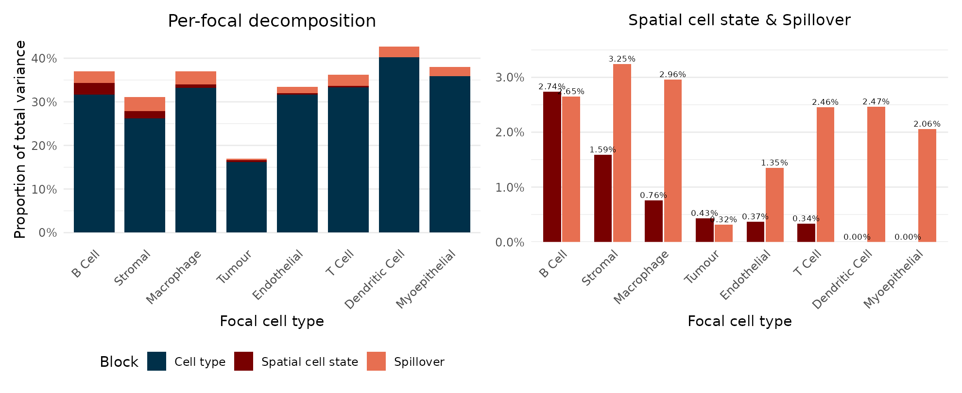
Beyond the dominant cell-type identity component, B cells, stromal
cells and macrophages carry the largest spatial cell-state
contributions, while dendritic and myoepithelial cells carry none on
this crop. The underlying per-gene table is available with
varianceDecomposition(fit).
Per-cell contamination
The spillover component above is a variance share per gene.
cellContamination() gives the per-cell view of the same
term: the loading rho_i and, more usefully,
contamFraction, the share of a cell’s expected counts
attributed to its local ambient field. A high fraction marks a cell
whose profile is largely explained by its neighbours rather than by its
own type, which is what a segmentation or transcript-assignment error
looks like.
cc <- cellContamination(fit)
head(cc, 3)
#>   cell   celltype        rho contamFraction
#> 1  442     Tumour 0.11504406    0.000000000
#> 2  444     B_Cell 0.00282706    0.001557513
#> 3  446 Macrophage 0.58779262    0.123800291
round(tapply(cc$contamFraction, cc$celltype, median), 3)
#>         B_Cell Dendritic_Cell    Endothelial     Macrophage  Myoepithelial
#>          0.091          0.083          0.018          0.073          0.038
#>        Stromal         T_Cell         Tumour
#>          0.038          0.072          0.000
Read the fraction rather than the loading. The ambient field is
cross-cell-type, so a cell with no differently-typed neighbour inside
the technical kernel has no ambient signal at all; its
rho_i is unidentified and shrinks to the empirical Bayes
prior mean, giving every such cell the same apparently middling loading.
On this crop that is most of the tumour interior:
zero <- cc$contamFraction == 0
c(cells = sum(zero), distinct_rho = length(unique(round(cc$rho[zero], 12))))
#>        cells distinct_rho
#>         4589            1
round(tapply(zero, cc$celltype, mean), 2)
#>         B_Cell Dendritic_Cell    Endothelial     Macrophage  Myoepithelial
#>           0.10           0.16           0.26           0.19           0.23
#>        Stromal         T_Cell         Tumour
#>           0.30           0.18           0.84
contamFraction reports those cells as zero, which is
correct; rho alone does not.
Pairwise spatial interactions
plotPairHeatmap() gives the percentage of each focal
type’s total variance contributed by spatial interaction with each
neighbour, computed as the focal’s spatial share split across neighbours
by a normalised Pratt attribution. Tumour as a
neighbour acts the most widely across the microenvironment,
reaching four focal types where no other neighbour reaches more than
two. The single strongest pair is B cells next to T cells.
plotPairHeatmap(fit)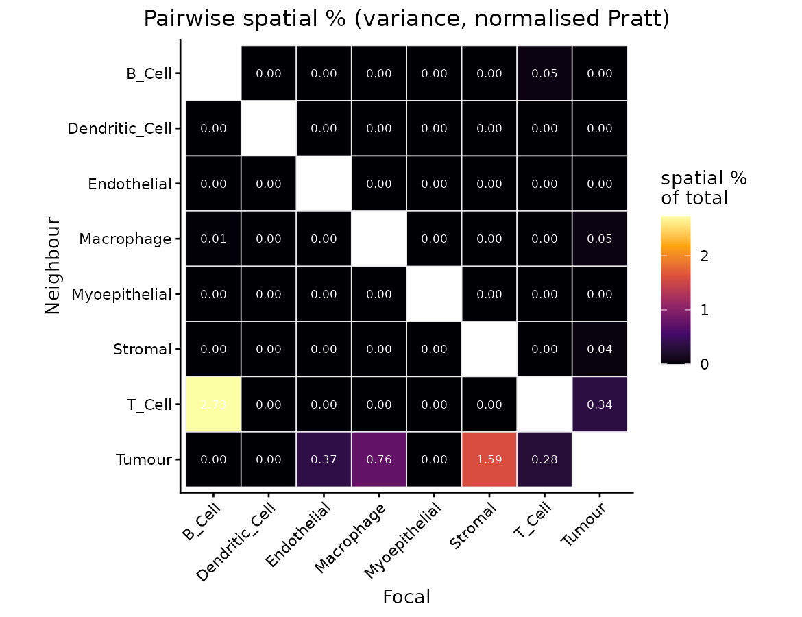
pairVariance() returns those same numbers as a long
table. The heatmap is drawn from it, so the two cannot disagree, and the
table is the easier thing to rank or pass on:
pairVariance(fit) |>
  arrange(desc(val)) |>
  head(5)
#> # A tibble: 5 × 3
#>   focal       neighbour   val
#>   <chr>       <chr>     <dbl>
#> 1 B_Cell      T_Cell    2.73
#> 2 Stromal     Tumour    1.59
#> 3 Macrophage  Tumour    0.756
#> 4 Endothelial Tumour    0.372
#> 5 Tumour      T_Cell    0.342
For a cohort with a condition, block = "responder" gives
the same attribution for the responder-by-proximity block rather than
the baseline spatial one.
Macrophage–tumour drivers
plotDrivers() ranks the genes mediating a relationship
by a driver score (combining the shrunken slope, its cell-type
specificity, and its expression level), alongside their per-gene
single-frame decomposition. For the macrophage-tumour pair, the top
drivers are the tissue-resident marker MRC1 (CD206),
reduced near tumour, and the lipid-associated marker
APOC1, elevated near tumour.
plotDrivers(fit, "Macrophage", "Tumour")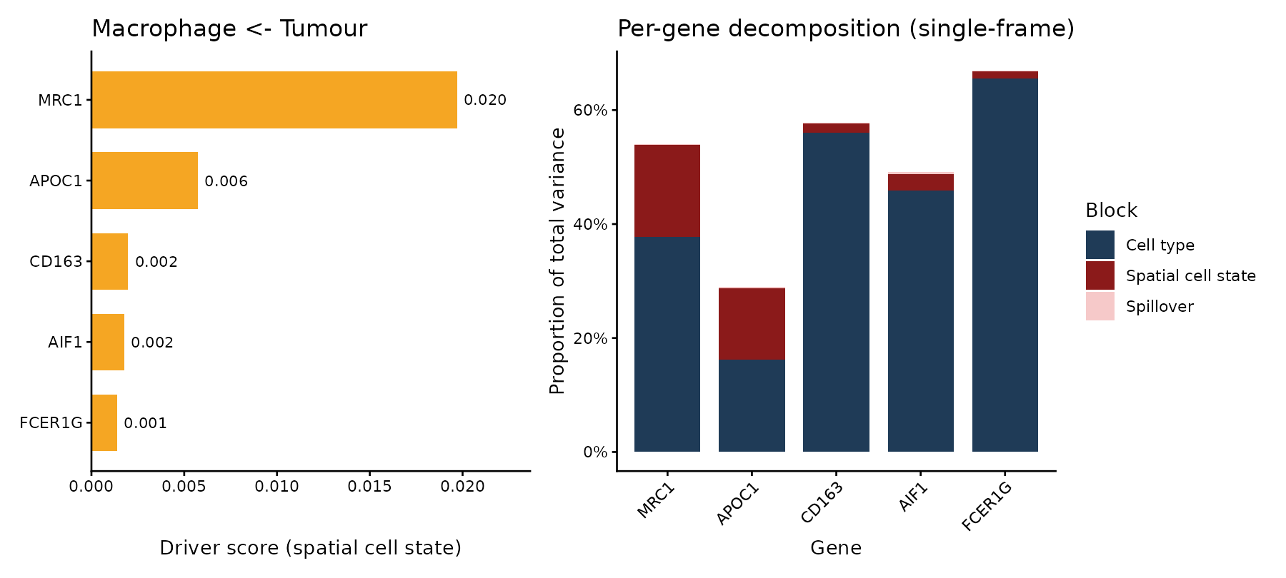
The shrunken slopes confirm the opposing directions:
neighbourSlopes(fit) |>
  filter(focal == "Macrophage", neighbour == "Tumour",
         gene %in% c("MRC1", "APOC1")) |>
  select(gene, estimate_shrunk, lfsr)
#>    gene estimate_shrunk         lfsr
#> 1 APOC1       0.1301689 1.077054e-17
#> 2  MRC1      -0.1494760 1.443290e-15
Visualising the proximity effect
plotProximity() bins each macrophage by its number of
tumour neighbours (within 30 um) and shows each gene’s raw counts per
bin. Because these genes are zero-inflated the box median sits at zero
in most bins, so the per-bin mean is overlaid as a point to make the
trend explicit. Macrophage MRC1 falls and APOC1 rises with tumour
proximity.
plotProximity(fit, spe, c("MRC1", "APOC1"), "Macrophage", "Tumour")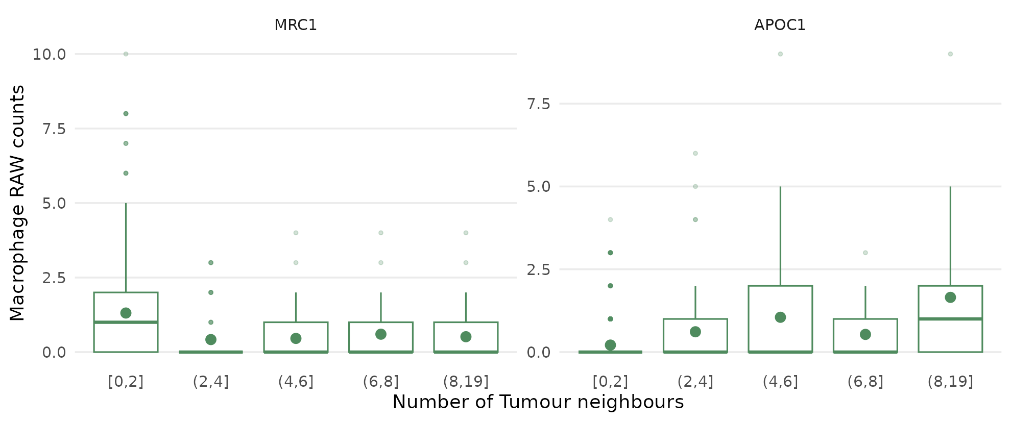
Biological interpretation
On this section PACE recovers a coordinated shift in macrophage state at the tumour interface: the tissue-resident marker MRC1 (CD206) is reduced and the lipid-associated, immunosuppressive marker APOC1 is elevated in macrophages near tumour cells. Because PACE separates this proximity effect from the transcript contamination that would otherwise inflate tumour-marker signal in the macrophages, the drivers it promotes are genuine macrophage genes rather than tumour genes bleeding across cell boundaries.
Saving a fit
A fit holds the fitted means and the contamination log-offset as full
cells x genes matrices. They make the object large: even
this small crop is
round(as.numeric(object.size(fit)) / 1e6, 1)   # MB
#> [1] 7.2
and a whole section runs to several hundred megabytes. They do not
have to be kept. paceDecompose() and
paceDrivers() read only per-cell-type summaries of the
fitted means, which the fit also stores, so a fit saved without the
matrices can still be re-decomposed (from the counts in
spe) and re-scored. (For an older fit saved without those
summaries, pass spe to both, and they are rebuilt exactly
from the fit and the counts.)
fit_small <- fit
for (nm in c("mu", "technical_offset_mat", "bleed_offset_mat"))
  fit_small@fit[[nm]] <- NULL
round(as.numeric(object.size(fit_small)) / 1e6, 1)   # MB
#> [1] 7.2
saveRDS(fit_small, "fit.rds", compress = "xz")Every readout above still works on the stripped fit, and re-decomposing it reproduces the table it already carries:
redone <- paceDecompose(fit_small, spe)
stored <- varianceDecomposition(fit)
num <- vapply(stored, is.numeric, logical(1))
max(abs(as.matrix(varianceDecomposition(redone)[num]) - as.matrix(stored[num])))
#> [1] 0
Session info
sessionInfo()
#> R version 4.6.1 (2026-06-24)
#> Platform: x86_64-pc-linux-gnu
#> Running under: Ubuntu 24.04.5 LTS
#>
#> Matrix products: default
#> BLAS:   /usr/lib/x86_64-linux-gnu/openblas-pthread/libblas.so.3
#> LAPACK: /usr/lib/x86_64-linux-gnu/openblas-pthread/libopenblasp-r0.3.26.so;  LAPACK version 3.12.0
#>
#> locale:
#>  [1] LC_CTYPE=C.UTF-8       LC_NUMERIC=C           LC_TIME=C.UTF-8
#>  [4] LC_COLLATE=C.UTF-8     LC_MONETARY=C.UTF-8    LC_MESSAGES=C.UTF-8
#>  [7] LC_PAPER=C.UTF-8       LC_NAME=C              LC_ADDRESS=C
#> [10] LC_TELEPHONE=C         LC_MEASUREMENT=C.UTF-8 LC_IDENTIFICATION=C
#>
#> time zone: UTC
#> tzcode source: system (glibc)
#>
#> attached base packages:
#> [1] stats4    stats     graphics  grDevices utils     datasets  methods
#> [8] base
#>
#> other attached packages:
#>  [1] tidyr_1.3.2                 dplyr_1.2.1
#>  [3] ggplot2_4.0.3               SpatialExperiment_1.22.0
#>  [5] SingleCellExperiment_1.34.0 SummarizedExperiment_1.42.0
#>  [7] Biobase_2.72.0              GenomicRanges_1.64.0
#>  [9] Seqinfo_1.2.0               IRanges_2.46.0
#> [11] S4Vectors_0.50.3            BiocGenerics_0.58.1
#> [13] generics_0.1.4              MatrixGenerics_1.24.0
#> [15] matrixStats_1.5.0           PACE_0.99.11
#> [17] BiocStyle_2.40.0
#>
#> loaded via a namespace (and not attached):
#>  [1] gtable_0.3.6        rjson_0.2.23        xfun_0.61
#>  [4] bslib_0.12.0        lattice_0.22-9      vctrs_0.7.3
#>  [7] tools_4.6.1         tibble_3.3.1        pkgconfig_2.0.3
#> [10] Matrix_1.7-5        SQUAREM_2026.1      RColorBrewer_1.1-3
#> [13] S7_0.2.2            desc_1.4.3          assertthat_0.2.1
#> [16] lifecycle_1.0.5     truncnorm_1.0-9     stringr_1.6.0
#> [19] compiler_4.6.1      farver_2.1.2        textshaping_1.0.5
#> [22] htmltools_0.5.9     sass_0.4.10         yaml_2.3.12
#> [25] pillar_1.11.1       pkgdown_2.2.1       jquerylib_0.1.4
#> [28] rmeta_3.0           cachem_1.1.0        DelayedArray_0.38.2
#> [31] dbscan_1.2.7        magick_2.9.1        abind_1.4-8
#> [34] tidyselect_1.2.1    digest_0.6.39       stringi_1.8.9
#> [37] mvtnorm_1.4-2       purrr_1.2.2         bookdown_0.48
#> [40] ashr_2.2-63         labeling_0.4.3      fastmap_1.2.0
#> [43] grid_4.6.1          cli_3.6.6           invgamma_1.2
#> [46] SparseArray_1.12.3  magrittr_2.0.5      patchwork_1.3.2
#> [49] S4Arrays_1.12.1     utf8_1.2.6          withr_3.0.3
#> [52] scales_1.4.0        rmarkdown_2.32      XVector_0.52.0
#> [55] otel_0.2.0          ragg_1.5.2          evaluate_1.0.5
#> [58] knitr_1.52          viridisLite_0.4.3   irlba_2.4.1
#> [61] rlang_1.3.0         Rcpp_1.1.2          mixsqp_0.3-54
#> [64] glue_1.8.1          BiocManager_1.30.27 jsonlite_2.0.0
#> [67] plyr_1.8.9          mashr_0.2.79        R6_2.6.1
#> [70] systemfonts_1.3.2   fs_2.1.0