Using PACE

The overview is the short version. This is the reference: what each readout gives you, the figures, and the handful of settings worth knowing about.

The readouts

pace_model — the model. One slope per (focal type, neighbour type, gene), with a per-cell contamination loading and gene-wise overdispersions. Given an AnnData it reads coordinates from obsm["spatial"], labels and condition from obs, gene names from var_names and counts from X or a layer, and never modifies it.

pace_shrink — which slopes to believe. Raw slopes are mostly noise. Multivariate adaptive shrinkage pools them, one mixture per neighbour type with the focal types as its conditions, and returns every slope with a local false sign rate. slopes.calls() reports how many effects are called and how many of those are expected to have the wrong sign.

pace_decompose — where a gene’s variance comes from. Per focal type and gene, split into cell-type identity, the baseline spatial effect, the condition-by-space interaction, contamination, and dispersion. Useful for the question “is this gene’s variation about where the cell is at all?” single_frame_decomposition gives the observed version, where the magnitudes are measured from the data and only the split within a cell type comes from the model.

pace_drivers — which genes carry a relationship. Per pair, genes ranked by b² · spec² · focal_mean. Squaring the slope makes the score direction-blind, so a gene pushed down ranks alongside one pushed up; specificity and expression level keep a barely-expressed gene off the top on a noisy slope. Filtered at lfsr < 0.05.

pair_variance — which neighbours matter to which cell types. Each focal type’s spatial variance split across its neighbours, so a row sums to that type’s spatial share and the own-type pair is excluded.

plot_* — five figures over the above.

Three more: build_neighbourhood() and ambient_field() return the kernels and the contamination field without fitting, for checking what the model is being given; anchor_genes() lists the genes that mark each type and so anchor its contamination; stash_pace() copies the readouts into adata.uns, and compact_fit() drops the rebuildable bulk from a fit you want to keep.

Figures

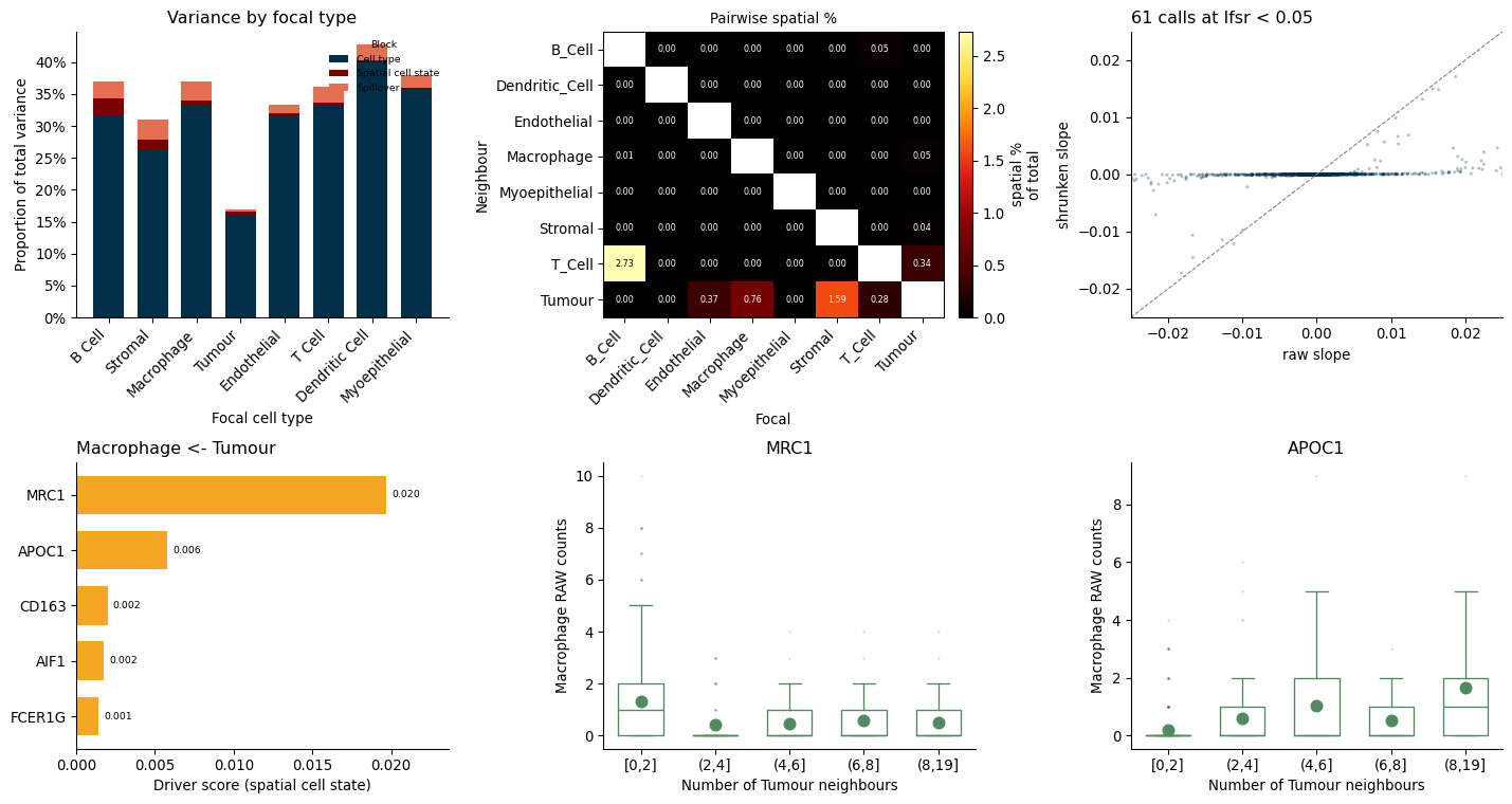
pace.plot_decomposition(frame)                 # full bar + the rescaled zoom
pace.plot_pair_heatmap(pairs, fit.cell_types)
pace.plot_drivers(drivers, "Macrophage", "Tumour", single_frame=frame)
pace.plot_proximity(fit, counts, ["MRC1", "APOC1"], "Macrophage", "Tumour")
pace.plot_shrinkage(slopes)

Two are worth knowing about. plot_decomposition leaves the residual block out, so its bars stop well short of 100%: the comparison is between the parts the model attributes, and a residual bar towering over the rest would tell you nothing. plot_drivers takes single_frame= to add a companion panel showing what each top gene’s variance is made of, which catches a gene that ranks highly because the focal type simply expresses a lot of it.

Every panel returns matplotlib axes, so saving is ordinary matplotlib. For publication, write PDF with Type 42 fonts, which keeps text editable and avoids the Type 3 fonts journals reject:

import matplotlib
matplotlib.rcParams["pdf.fonttype"] = 42
axis, zoom = pace.plot_decomposition(frame)
axis.figure.savefig("decomposition.pdf", bbox_inches="tight")

Things worth setting

Give it counts. adata.X holds whatever the last preprocessing step left there, and a negative binomial fit of log-normalised values will converge and report slopes that mean nothing. Non-integer values are refused; point layer at the raw counts.

Name the reference arm of a condition. Its first level is what every other arm is contrasted against, so it decides what the baseline slopes mean and which way the interaction points — this is not a relabelling. Leaving condition_levels unset picks one for you and warns.

fit = pace.fit_anndata(adata, "cell_type", condition_key="Responder",
                       condition_levels=["non-responder", "Responder"])

kernel_per_image is False: the neighbour search runs across the whole object even when it has several images, which is what fields of view from one section want. Set it True when the images are genuinely separate samples.

types= fixes the cell type order, and so the row order of everything downstream. The default sorts the observed labels.

ambient_mode="stream" avoids materialising the cells-by-genes contamination field, which runs to several GB at a million cells. It is a memory setting and nothing else — the fit is identical either way.

On a condition fit, pace_shrink returns the responder layer, the condition-by-neighbour interaction, not the baseline proximity effect.

Tests

pip install -e ".[test]"
python -m pytest tests

From a non-editable install, run them from outside the checkout (cd /tmp && python -m pytest /path/to/pace-python/tests): the repository root holds the source package pace/, which shadows the installed one but has no compiled _core, and the resulting ImportError blames a circular import rather than the real cause.

Building from source

Two things are not free choices.

Eigen must be 3.4. Later majors vectorise and reduce in a different order, which moves the fitted effects by about 3e-4, so the build refuses them:

bash tools/fetch_eigen.sh && EIGEN_INCLUDE_DIR=$PWD/eigen-3.4.0 pip install -e .

PACE_ALLOW_ANY_EIGEN=1 builds anyway. Installing a released wheel avoids the question entirely.

On macOS, use Apple’s toolchain. A conda or Homebrew clang brings an old ld64 that links a shared object which loads nowhere — the build succeeds and it fails at import with mis-aligned LINKEDIT string pool:

CC=/usr/bin/clang CXX=/usr/bin/clang++ \
  LDSHARED="/usr/bin/clang -bundle -undefined dynamic_lookup" pip install -e .

ld -v should report PROJECT:ld-27037 or newer.